I’ve recently become interested in building a digital guitar pedal. Specifically, I want to build a one-knob talking filter that would sound a bit like this:
The talking effect comes from a formant filter being modulated in response to notes. To detect notes, I need a transient detector, a device that identifies rapid changes in audio amplitude or spectral content. Rather than allowing users to select these parameters (and compromise my minimal one-knob aesthetic), I used a learning algorithm to select a set of parameters based on data. This design is functionally a machine learning model with a less general set of basis functions. Compared to traditional ML techniques for signal processing, such as CNNs or LSTMs, this approach has the following advantages:
- Predictability: An audio effect that doesn’t do what the musician expects every time is worthless. Simpler models are less likely to overfit and even when the model is wrong, it will always be wrong in similar circumstances.
- Decreased resource utilization: My transient detector needs to run on an ESP32-S3 and still leave room for the main DSP algorithm, such as the filter effect. Using only 18 parameters and being based on conventional DSP techniques, it is possible to manually optimize the implementation for the most efficient resource usage.
- Less training data: Since this is a one-person hobby project, I didn’t want to spend a lot of time labeling training data. I manually labeled about 6 minutes of audio, which only took me a couple of hours.
- Explainability: Because the model is forced to take the shape of a classical algorithm, the learned parameters are directly interpretable and are always in real-world units (i.e., seconds or hertz).
- Global Optimization: Complex ML models are constrained to using local-minima search algorithms such as gradient descent. A very small model can be trained with global optimization techniques that take advantage of the whole parameter set.
The downside is accuracy, with my model achieving around 60% to 70% precision with similar recall. This may be due to the model’s limited ability to analyze frequency domain content of the input, something traditional models are more suited to.
Model Architecture
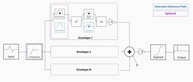
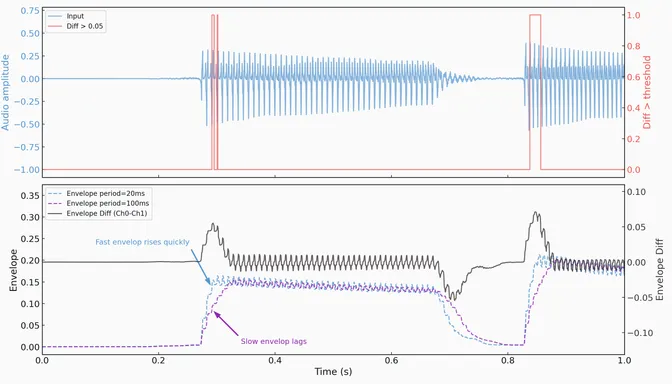
The classic transient detector algorithm uses a fast envelope generator and a slow envelope generator, which are subtracted to produce an estimate of how quickly the amplitude of the original signal is changing. When the input amplitude changes quickly, this difference exceeds a threshold and a note is detected.
My model also uses a bank of envelope generators to estimate the signal’s amplitude, although the quantity is configurable rather than being fixed at two. Rather than differencing and thresholding the output, the model weights each envelope, sums them, and limits the output with a sigmoid function. By selecting appropriate weights and biases, the model is able to mimic the effect of the classical algorithm, although this architecture is more flexible. Replacing the threshold with a sigmoid function allows the model to be differentiable. For differentiability, the moving average is replaced by a smoothed version during training, but the simple moving average is retained during inference.
Two optional components are added to the model, enabled by hyperparameters. The first is an audio compressor, which helps normalize the overall level of the input. The time constant of the compressor’s internal envelope generator, the threshold, and the makeup gain are learnable parameters.
The second optional component is a per-channel bandpass filter to allow each envelope to focus on a specific region of the audio spectrum. Each filter has a learnable center frequency and Q (which controls the bandwidth). They are implemented as biquad IIR filters to allow for efficient inference on a microprocessor. However, this filter design is inefficient on a GPU, so, during training, an equivalent FIR filter is used.
Data & Learning
For training data, I used a collection of free stems, including recordings of guitar (both DI and distorted), kick drum, bass, and synthesizer. I listened for the start of each note and labeled it in Audacity. These labels are used to create a target signal which is zero everywhere except for the period starting at each transient and lasting 20ms, where it is one. The model attempts to reproduce this target signal.
To optimize the parameters, traditional optimization techniques such as stochastic gradient descent and L-BFGS-B tend to stay too close to the initial conditions. Furthermore, these techniques don’t work well with differently scaled parameters, such as the filter cut-off (in hertz) and envelope time (in seconds). To solve this, I used global optimization techniques. Both basin-hopping with an analytic Jacobian and differential evolution were evaluated, with differential evolution giving the best results. Unlike stochastic gradient descent, these global optimization techniques require the entire training set to be included in a single batch. As the whole of the training data is only twenty 5-second audio clips, this is not a problem.
Results
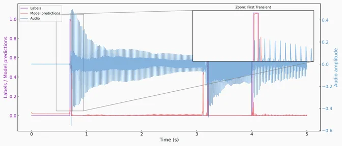
I evaluated the model on a selection of audio clips not included in the training data. Rather than comparing to the target signal, the evaluation metrics are based on the phenomenon of interest, detecting a transient. Predictions are created from a rising edge detector with hysteresis on the model output and compared to ground truth. If a detection is within 20ms of the true value, a true positive is reported. If the detection is not within that window, a false positive is reported. Similarly, false and true negatives are computed.
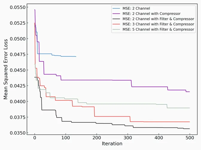
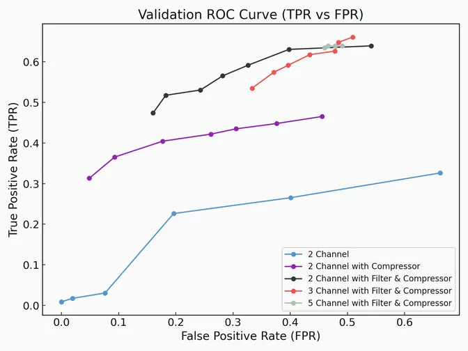
Overall, the model performed modestly, achieving 70% precision at 53% recall for the three-channel with compressor and bandpass filter case. Interestingly, increasing model complexity mostly assists with recall and not precision. I believe this is attributable to “hard” transients which involve a change in pitch without an accompanying change of amplitude. I did not use separate validation and test sets, partly because the design of the model is robust to overfitting, but more because this is a personal project and I did not want to spend too much time labeling data.
The model generalized well enough to produce the audio clip at the beginning of this post. Future work involves improving model performance with a more advance architecture and implementing and profiling the design on hardware.
Call to action: If you would be interested in a series of well-tuned one-knob pedal effects that are always in the sweet-spot, reach out to me. They say it’s never to early to start doing market research, although I don’t have plans to commercialize any time soon.